Introduction

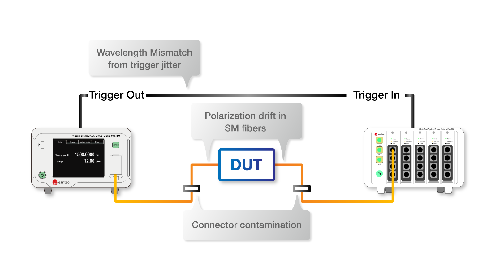
Optical power measurement is a dependency for most photonics test workflows, including component characterization, subsystem integration, and production screening. In high-volume environments, the dominant failure modes are rarely “meter broken.” They are typically workflow-level: unstable reference conditions, wavelength/polarization mismatch, connector contamination, drift between reference and test states, or untracked setup changes.

When power measurement is used to compute insertion loss, gain, or pass/fail thresholds, small systematic biases can shift yield classification and process capability metrics. The practical requirement is not only a calibrated optical power meter, but a measurement chain that is stable, repeatable, and auditable across operators, stations, and time.

This paper focuses on: (1) what the instrument reports, (2) how detector physics drives error terms, (3) calibration meaning and limits, and (4) test-setup controls that scale to manufacturing use cases, including automated logging and periodic verification. 

What Is Being Measured

Optical Power vs Optical Energy

Optical power is the rate of energy transfer (W). Optical energy is the time integral of power (J). Many fiber optic test applications use continuous wave (CW) or quasi-CW signals where power is the controlled and reported quantity.

For modulated signals, an optical power meter reports average power over its integration time. Peak power, modulation depth, and waveform features require separate measurement methods.

Units Engineers Actually Use: W, dBm, dB

W / mW / µW: Absolute power in physical units.

dBm: Absolute power expressed on a logarithmic scale referenced to 1 mW.

• P(dBm)=10log10(P(mW))
• P(mW)=10P(dBm)10

dB: A ratio between two power levels (relative measurement). dB is not an absolute unit.

Insertion loss and gain are typically computed in dB.

A common workflow error is mixing dBm (absolute) and dB (relative) without explicitly defining the reference state and measurement plane.

Absolute vs Relative Power Measurements

Absolute power measurement determines optical power at a defined measurement plane, referenced to traceable calibration. It is required when verifying transmitter output, establishing power budgets, or meeting test requirements specified in physical units.

Relative power measurement evaluates change between two states and is typically expressed in dB. Insertion loss and gain measurements often use a reference normalization step so that some systematic terms cancel. Cancellation depends on conditions:

• The reference and test states must be matched in wavelength content and polarization behavior.
• The measurement chain must remain stable between the reference capture and the test reading.
• Linearity and repeatability must be adequate over the power range used.

If reference and test states differ in wavelength content or polarization state, wavelength-dependent responsivity and polarization-dependent effects introduce differential errors that do not cancel. In that case, results depend more strongly on sensor characterization and calibration validity.

How Optical Power Meters Work

Detector Technologies

Optical power sensors use thermal detection or semiconductor photodiode detection. Detector type affects response time, wavelength dependence, sensitivity, and drift mechanisms.

Thermal Detectors

Thermal detectors convert incident optical radiation to heat and measure the temperature change. The conversion is not wavelength-selective in principle, so thermal detectors are used when reduced wavelength dependence is needed. Practical performance depends on absorption characteristics of the detector surface and coatings.

Response time is governed by thermal mass and heat flow (typically milliseconds to seconds). Sensitivity is generally lower than photodiode sensors, and minimum detectable power depends on design and environment. Thermal detectors are sensitive to ambient temperature variation, airflow, and mechanical conditions that affect heat exchange. Surface contamination or coating damage changes absorptivity and therefore calibration.

Semiconductor Photodiodes

Photodiodes generate current proportional to incident optical power. These sensors are widely used in fiber optic testing due to fast response and high sensitivity.

Photodiode responsivity (A/W) depends on wavelength because absorption depth, quantum efficiency, and junction behavior vary with photon energy. Material choice sets the usable wavelength range. Silicon photodiodes cover visible to near-infrared with cutoff near 1100 nm. InGaAs photodiodes extend sensitivity into the near-infrared wavelengths used in telecom and datacom.

At high power, saturation mechanisms, series resistance effects, and heating reduce linearity. At low power, dark current and electronic noise become significant. Usable dynamic range depends on detector area, amplifier design, and bandwidth.

Quick Selection Guide (Technical Fit, Not Buying Advice)

Use-case-driven selection reduces error terms that cannot be removed later by averaging.

This table is about measurement physics and workflow constraints. It does not replace instrument-specific performance verification.

Responsivity and Wavelength Dependence

An optical power meter converts detector output into a power reading using calibration factors. For photodiode-based sensors, wavelength-dependent responsivity is a primary correction term.

If the meter wavelength setting does not match the actual wavelength content, the reported value is biased by responsivity mismatch. This risk is common when switching between standard wavelengths (e.g., 850 nm multimode contexts vs 1310/1550 nm single-mode contexts) or when measuring sources with uncertain wavelength.

Meters apply corrections using discrete tables or interpolation. Residual error depends on calibration data quality, interpolation method, and stability of detector spectral response.

For broadband sources, uncertainty increases unless the spectrum is characterized and a weighted correction is applied, or a detector with reduced wavelength dependence is used for the band of interest.

Calibration: What It Means and What It Does Not

Calibration Traceability

Calibration establishes the relationship between indicated value and optical power realized by a reference standard maintained through a traceability chain. In the United States, traceability is referenced to NIST; other countries maintain equivalent national metrology institutes.

A calibration certificate documents comparison between the device under test and a reference standard under stated conditions.

Typical content includes:

• Deviations at specified wavelengths and power levels
• Uncertainty associated with the calibration process
• Environmental conditions during calibration
• Calibration date and recommended recalibration interval

What calibration does not guarantee:

• It does not ensure the meter stays in specification between calibration events. Responsivity drift, mechanical changes, and electronic aging can alter results before the next scheduled calibration.
• Calibration at one wavelength does not establish accuracy across all wavelengths unless multi-wavelength characterization is included and the wavelength correction remains valid.
• Calibration does not control user-induced errors (connector contamination, fiber handling, alignment sensitivity, environmental instability).

Calibration Interval Under Utilization Pressure

Calibration interval selection depends on required uncertainty, utilization level, and exposure conditions. In high-usage environments, practical risk increases due to:

• Higher connector mating cycles and adapter wear
• Higher probability of surface contamination
• Larger temperature variation across stations
• More frequent configuration changes (wavelength, power range, fixtures)

A common scalable approach is to treat calibration as a layered control: 

• Formal calibration at defined intervals 
• Interim verification using a transfer standard (stable source or reference artifact) 
• Station-level controls (logging and drift detection) to detect out-of-family behavior early 

Transfer Standards and Verification Logic 

Interim verification uses a transfer standard to track changes in the measurement chain over time. The goal is not to “recalibrate in-house,” but to detect drift, damage, or setup deviation. 

A verification routine should define: 

• The measurement plane and connection sequence 
• Allowed variation band (defined by internal uncertainty targets) 
• Logging of environmental and configuration metadata (wavelength setting, range, attenuator state, adapter ID if controlled) 

Accuracy, Repeatability, and Uncertainty 

Accuracy vs Repeatability 

Accuracy is closeness of a measurement result to the reference value under defined conditions. It is limited by systematic errors and the uncertainty of the calibration and method. 

Repeatability is the dispersion of results under nominally identical conditions over a short interval. High repeatability does not imply low systematic error. 

Example 

A meter can be repeatable but biased (systematic offset). It can also appear accurate on average while being unstable due to connection or environment variability. 

For insertion loss, repeatability and stable reference conditions often dominate. For absolute verification tasks, systematic bias control and repeatability are both required. 

Dominant Uncertainty Sources in Production-Like Setups 

Connector repeatability and cleanliness 

Coupling variation with each mate/unmate cycle is often a dominant term. Wear state, contamination, and handling method matter more in practice than nominal connector type. 

Polarization effects 

If polarization is not controlled, sensor PDL and stress-induced polarization changes introduce variation. Mitigation includes low-PDL sensors, polarization scrambling (where compatible), or polarization-maintaining components when fixed polarization is required. 

Temperature and ambient conditions 

Photodiode responsivity and electronics drift with temperature. Thermal detectors additionally respond to airflow and gradients. Stray light leakage creates offsets that are significant at low power. 

Range selection, attenuation, and linearity behavior 

Operating near limits increases the influence of noise (low power) or nonlinearity/saturation (high power). Attenuation may be required to keep power in a stable operating region, but attenuation devices introduce their own uncertainty and should be treated as part of the measurement chain. 

Standard Optical Test Setup for Insertion Loss (Bench and Scalable Variants) 

Reference Power Setup (Normalization) 

A reference reading represents optical power delivered through a defined reference path. A typical normalization sequence is: 

1. Connect source to power meter using a reference jumper with clean, inspected connectors 
2. Configure the meter for the correct wavelength 
3. Allow the system to stabilize 
4. Record the reference power 
5. Insert the device under test without disturbing key connections where possible 
6. Measure transmitted power 
7. Compute insertion loss from transmitted/reference power ratio 

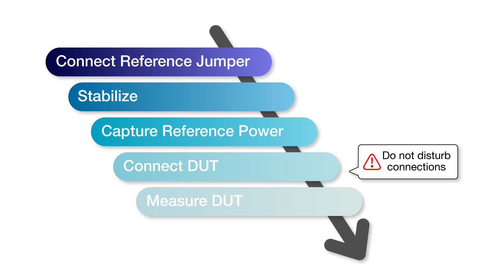
Control objective: maintain consistent connections between reference and measurement states. Reconnecting the reference path adds connector repeatability terms.

Where an Optical Attenuator Fits (and Why)

Attenuators are used to keep power within a stable operating region of the sensor and front-end electronics, and to avoid saturation in photodiode sensors at higher powers. When an attenuator is inserted, it becomes part of the measurement chain:

• its insertion loss must be stable over time and handling
• its wavelength dependence and return loss behavior can affect results
• it can change polarization behavior in some setups

For scalable workflows, attenuator state (in/out, set value if variable) should be recorded as configuration metadata.

Connector and Fiber Handling Checklist

• Inspect endfaces before measurement
• Clean using a defined process (dry and wet steps as needed)
• Use consistent mating technique and coupling torque / latch engagement
• Track wear-critical adapters and limit unnecessary mate cycles
• Maintain stable routing; avoid movement during reference/test transitions

Environmental Controls That Matter at Scale

• Reduce airflow and temperature gradients at the setup
• Keep stations away from HVAC vents and localized heat sources
• Reduce vibration coupling; use stable fixtures
• Control ambient light; ensure connections are light-tight for low-power measurements

Common Measurement Errors and How to Avoid Them

Wavelength mismatch

Error: Incorrect wavelength setting produces systematic bias due to responsivity mismatch.

Avoidance: Verify wavelength when uncertainty is material. Use correct wavelength configuration. For broadband sources, apply spectrum-aware methods or use a suitable detector approach for the band of interest.

Power range and linearity misuse

Error: Operation near range limits increases noise influence or nonlinearity effects.

Avoidance: Keep measurements within a stable operating region. Use attenuation when needed. If linearity is critical, perform a controlled power step check using a stable source and known attenuation steps to confirm proportional response over the range used.

Back reflections

Error: Reflections can alter source output stability (source-dependent) and create interference effects at the detector input.

Avoidance: Use practices that reduce reflections (e.g., APC where compatible), isolate reflection-sensitive sources, and control connector condition. Apply additional reflection control based on observed instability.

Polarization sensitivity

Error: Uncontrolled polarization changes introduce reading variation when sensor or path is polarization dependent.

Avoidance: Use low-PDL sensors where polarization is uncontrolled, apply polarization scrambling where compatible, or use polarization-maintaining components when fixed polarization is required.

Calibration status ignored

Error: Operation beyond calibration intervals or without interim verification increases the risk of unbounded systematic error.

Avoidance: Implement calibration management and periodic verification. If results shift unexpectedly, verify the measurement chain before attributing deviation to the device under test.

Insufficient stabilization

Error: Drift between reference and test readings due to warm-up or thermal transients.

Avoidance: Allow stabilization consistent with the setup. Observe readings for stability before capturing the reference.

Application Examples (Manufacturing-Relevant)

Component Characterization Across Standard Wavelengths

Characterization often requires multi-wavelength measurement (e.g., 1310/1550 nm for single-mode components, or 850 nm for multimode contexts). Multi-wavelength workflows increase the chance of wavelength-setting mismatch and require consistent reference capture at each wavelength.

High-Volume Insertion Loss Screening

High-volume screening emphasizes procedural control: reference stability, connector hygiene, configuration tracking, and drift detection. Automation can reduce operator variability but adds components that must be verified as part of the chain (switches, patch panels, fixtures).

Wafer-/Probe-Adjacent Measurement Chains

Probe-station-adjacent setups add alignment sensitivity, environmental gradients, and repeated connect cycles. The dominant error terms often shift toward mechanical stability, repeatable coupling conditions, and systematic drift tracking over time.

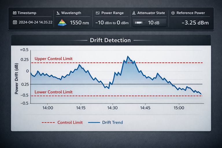
Data Logging and Drift Detection

For scalable operations, logging should include at least:

• wavelength setting
• power range
• attenuator state
• reference power value and timestamp
• environmental context when available (temperature)

This allows drift detection and correlation before yield metrics shift.

Summary and Practical Takeaways

• Optical power measurement quality is determined by detector behavior, calibration validity, and test setup control.
• In high-volume environments, dominant risks are workflow-level: reference instability, connector variability, configuration drift, and untracked changes.
• Calibration provides a traceable relationship under specified conditions, but it does not remove setup-induced errors or guarantee stability between events.
• Scalable measurement control combines calibration management, interim verification, and station-level drift detection with consistent procedures.

When absolute accuracy is required

• Transmitter output verification, power budgets, and requirements specified in physical units
• Requires traceable calibration, controlled measurement plane definition, correct wavelength configuration, and management of systematic error terms

When repeatability dominates

• Insertion loss screening and comparative measurements under controlled reference conditions
• Requires stable reference capture, controlled connections, and drift monitoring

Workflow controls that scale

• Define measurement planes and connection sequences
• Track configuration state (wavelength, range, attenuation)
• Apply connector inspection/cleaning and wear management
• Use verification routines to detect drift before it impacts yield or long-term trends